Building a survivor curve from observed data
Tags:
#Teaching
#Duration Modeling
#R
#Survival Function
A few weeks ago we were asked to teach the basics of (interpreting) duration models to a group of consumers without using any math. When I learned about this it involved a lot of math and Stata, and when you look around the web it’s usually presented similarly. So this was a bit of a challenge.
A nice thing about duration analysis though is that a lot of the key concepts are already explicitly graphical, like survival curves (wikipedia) and hazard rates. Below, for example, is a survival curve for cancer patients diagnosed with acute lymphoblastic leukemia between 1988 and 2008 in the US, from SEER fast stats:
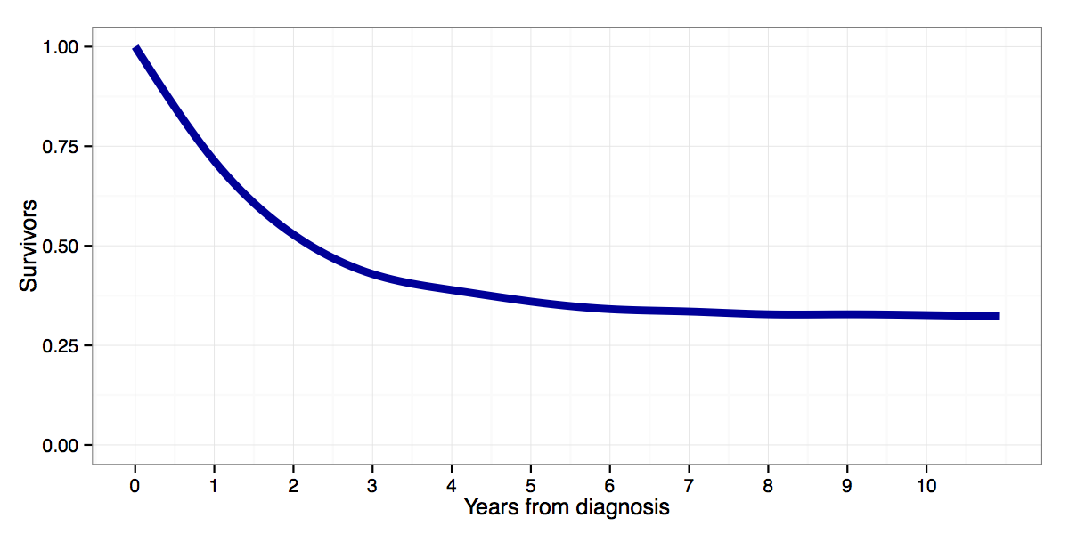
Starting from the moment at which a patient is diagnosed with cancer (year 0), it shows the proportion of patients who survive without relapse or death any given number of years from diagnosis. Two years from diagnosis, 50 percents of patients are still event free. Five years from diagnosis about 35 percent are event free (what you might call cured), etc. Alternatively, one could interpret it as the probability that a given ALL patient will be alive 2 or 5 years from diagnosis, with probabilities of 0.5 and 0.35 respectively.
So far so good, except that in practice one has to estimate survival functions on the basis of limited empirical data, e.g. using a Kaplan-Meier estimate (wikipedia). The resulting estimated survivor curves are not smooth like the curve above, but ragged. Using another example of lightbulbs, with data for the number of days until five bulbs burned out, one might get something like this:
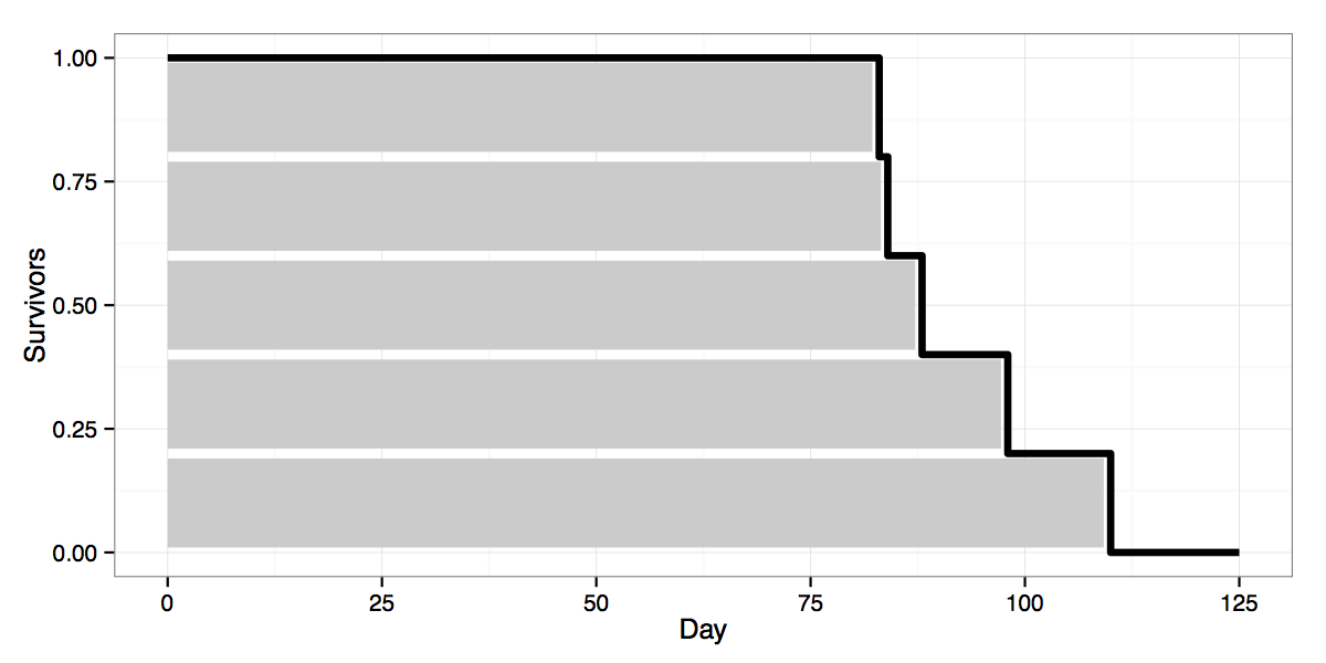
The black line shows the survivor curve estimate, based on data for the five lightbulbs. I added the grey bars to represent the number of days each of the five bulbs lasted to show how the survivor estimate is built up from individual failures. E.g. the top bar is the first bulb, which lasted for ~80 days. Thus on day 25 all 5 bulbs are still burning and our survivor curve is at 1.0. Around day 80, after the first bulb has failed, 4 of 5 or 0.8 of the original bulbs are still “alive”, bringing the curve down to 0.8. And so on for each additional failure.
Taking a cue from Bayesian Biologist’s video of Bayesian updating, and Drew Conway’s video of Chicago crime , I thought it would be nice to create a video that shows how an empirical survivor curve like this is built up from observed failure data, and how it changes as you add more data.
First, a simple backstory: Imagine you move into a new apartment, and having an obsession with measurement, you start keeping track of how long the lightbulbs in your five light fixtures last (it’s a small apartment). In the video below, the top half shows the five fixtures, where each bar represents a lightbulb and the number of days it is in operation now. On day 0 all 5 fixtures have new bulbs, i.e. there are no failures yet. Thus the survivor curve estimate, shown at the bottom, is not very useful (we disregard bulbs that haven’t burned out yet, i.e. no censoring).
Time goes by and after 80 days bulbs are starting to burn out. With data on failures we can now start updating our survivor curve to reflect those failures. The first updates still leave us with a very rough survivor curve estimate, but as more bulbs fail the curve starts getting a nicer shape. Note also that the mean time to failure (MTTF) in the bottom left corner starts getting closer to it’s theoretical value. The video ends after a year’s worth of simulation, but the longer we let it run the smoother the KM estimate would get. Eventually the KM estimate should converge to the theoretical survivor curve shown in red at the end of the video.
I created the video using R, with the code below. You’ll need ffmpeg to combine the individual frames into a video at the end.
library(ggplot2)
library(gridExtra)
## functions for simulated dgp
createSurvivalFrame <- function(f.survfit) {
## Create data frame to pass to ggplot2 using survfit result
if (class(f.survfit)!='survfit') stop('Need &quot;survfit&quot; class object.')
f.surv <- data.frame(time=f.survfit$time, surv=f.survfit$surv)
f.start <- data.frame(time=c(0, f.surv$time[1]), surv=c(1, 1))
# add row at end (0 to end of time)
f.end <- data.frame(time=125, surv=0)
f.surv <- rbind(f.start, f.surv, f.end)
return(f.surv)
}
qplot_survival <- function(f.surv) {
require(ggplot2)
p - ggplot(data=f.surv) + geom_step(aes(x=time, y=surv), direction='hv', lwd=1.5)
p <- p + theme_bw() + ylim(c(0, 1)) +
scale_x_continuous(breaks=c(0, 25, 50, 75, 100, 125), limits=c(0,125)) +
labs(y='Survivors', x='Day')
return(p)
}
## function to simulate lightbulbs
lights_sim <- function(max.days=100) {
require(survival)
require(ggplot2)
require(gridExtra)
# Initalize
obs.bulbs <- NULL
fixtures <- data.frame(no=1:5, bulb=NA, bulb.life=NA, bulb.spell=0, event=F)
bulb <- 0
true.mttf <- round(gamma(1+1/10)*100)
mttf <- 'NA'
# Initial survival plot
f.surv <- data.frame(time=c(0, 125), surv=c(1, 1))
p <- qplot_survival(f.surv) +
annotate('text', x=0, y=0.2, hjust=0,
label='Estimated MTTF:', size=4) +
annotate('text', x=35, y=0.2, hjust=0,
label=mttf, size=4) +
annotate('text', x=0, y=0.1, hjust=0,
label='Theoretical MTTF:', size=4) +
annotate('text', x=35, y=0.1, hjust=0,
label=true.mttf, size=4)
# Simulate through max.days
for (day in 1:max.days) {
# Update spell counters, reset events
fixtures$bulb.spell <- fixtures$bulb.spell + 1
# Place bulbs in empty fixtures
while (any(is.na(fixtures$bulb))) {
bulb <- bulb + 1
fixtures[match(NA, fixtures$bulb), c('bulb', 'bulb.life')] <- c(bulb, round(rweibull(1, shape=10, scale=100)))
}
# Check for bulbs to burn out now
fixtures$event <- with(fixtures, ifelse(bulb.life==bulb.spell, T, F))
if (any(fixtures$event)) {
obs.bulbs <- rbind(obs.bulbs, fixtures[fixtures$event==T, c('bulb', 'bulb.life', 'event')])
fixtures[fixtures$event==T, c('bulb', 'bulb.life', 'bulb.spell', 'event')] <- matrix(rep(c(NA, NA, 0, F), sum(fixtures$event)), ncol=4, byrow=T)
# Mean time to failure estimate
mttf <- round(mean(obs.bulbs$bulb.life), digits=1)
# Kaplan-Meier surv curve
surv.data <- with(obs.bulbs, Surv(bulb.life, event))
f.surv <- createSurvivalFrame(survfit(surv.data ~ 1, surv.data))
p <- qplot_survival(f.surv) +
annotate('text', x=0, y=0.2, hjust=0,
label='Estimated MTTF:', size=4) +
annotate('text', x=35, y=0.2, hjust=0,
label=mttf, size=4) +
annotate('text', x=0, y=0.1, hjust=0,
label='Theoretical MTTF:', size=4) +
annotate('text', x=35, y=0.1, hjust=0,
label=true.mttf, size=4)
}
# fixture plot for each day
p.fix <- ggplot(data=fixtures) +
geom_bar(aes(x=factor(no), y=bulb.spell), fill=rgb(0,0,0.61), width=0.3) +
scale_y_continuous(limits=c(0, 125), name='', breaks=c(0, 25, 50, 75, 100, 125)) +
scale_x_discrete(name='Lamp') + coord_flip() + theme_bw() + theme(axis.title.y=element_text(vjust=0.1)) +
theme(plot.margin=unit(c(1,1,0.1,1.45), 'lines')) + ggtitle(paste0('Day: ', day))
# Plot frames for each day
png(paste0('graphics/frames/', sprintf('%03d', day), '.png'))
grid.arrange(p.fix, p)
dev.off()
# Progress bar
pb <- txtProgressBar(min=0, max=max.days, style=3, width=50)
setTxtProgressBar(pb, day)
}
## Add last frame with true survivor curve
# unobserved data-generating process
dgp <- data.frame(t=1:125, f=dweibull(1:125, shape=10, scale=100))
dgp$F <- cumsum(dgp$f)
dgp$S <- 1 - dgp$F
true <- p + geom_line(data=dgp, aes(x=t, y=S), col='red', lwd=1, linetype='dashed') +
annotate('text', label='Empirical', x=70, y=0.65) +
annotate('text', label='Theoretical', x=105, y=0.72)
png(paste0('graphics/frames/', sprintf('%03d', max.days+1), '.png'))
grid.arrange(p.fix, true)
dev.off()
# done, return failures
return(list(obs = obs.bulbs, current = fixtures, dgp = dgp))
}
### End of functions ###
## Simulate
set.seed(1152359)
sims <- lights_sim(365)
system('ffmpeg -f image2 -r 10 -i ~/path/to/frames/%03d.png ~/path/to/video/lightbulbs.mp4')